Using the workbench

The workbench is a full GIS workspace in a browser tab. Saved services become live map layers, your own files sit alongside them, and the analysis results chain into further analysis. It is free, and it needs no account.

Opening it

Click the Geo Hound toolbar icon, then Open Workbench in the popup. It opens in a new tab. That is the only way in: there is no context-menu item and no keyboard shortcut.

The layout

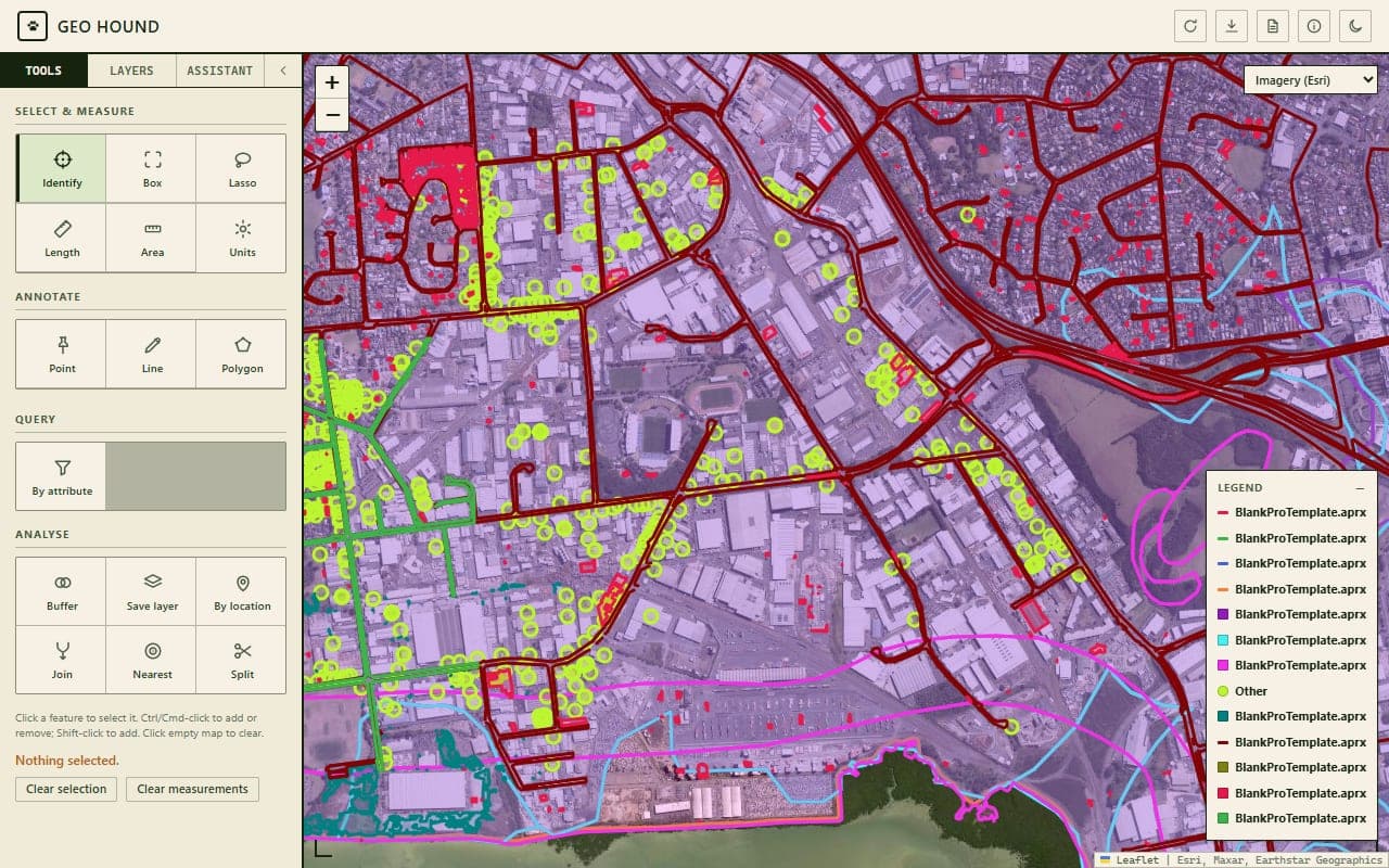
Three things to know about the furniture:

• The rail, on the left, has three tabs: Tools, Layers, and Assistant. The Assistant tab is the one open when the workbench loads.
• The map fills the middle, with a basemap picker top-right and a legend bottom-right.
• The dock slides up from the bottom to show attribute tables. It is hidden until you open a table or select something.

The top bar carries three icon buttons: export the map as PNG, export a PDF map report, and the theme toggle.

Adding a saved service as a layer

Open the Layers tab. Every service the detector has saved appears as a card. Click Add to map.

One thing worth understanding, because it surprises people: for vector services, Geo Hound fetches only the features in your current map view, not the whole dataset. You will see "Fetching features for current view...", then "Added N features." If you get "No features in the current view. Pan/zoom and try again.", the data is somewhere else on the map.

If the layer is truncated by the server's per-request cap, a Fetch all button appears on the card. That pages through the entire dataset, which is what you want before running analysis on the whole thing.

Each card is badged so you can see what you are dealing with: VECTOR, RASTER, RESULT, IMPORT, or UNKNOWN. Rasters are view-only; you cannot run analysis on them.

Importing your own files

Click Import file... in the Layers tab, or just drag the file anywhere onto the page. You can drop several at once.

The accepted formats are GeoJSON, JSON, CSV, KML, KMZ, GPX, and a zipped shapefile.

Two practical constraints:

• GeoJSON must be in WGS84. A file declaring any CRS other than CRS84 or EPSG:4326 is rejected. Reproject it first.
• CSV needs latitude and longitude columns, named something recognisable: lat, latitude, or y for one, and lon, lng, long, longitude, or x for the other. Otherwise you get "No latitude/longitude columns found".

Files over 20 MB, or layers over 50,000 features, ask for confirmation first.

The layer card

Each vector layer card carries:

• a colour swatch that opens a twelve-colour palette;
• Add to map / Remove from map;
• Hide / Show;
• Open table;
• a Download... menu: GeoJSON, KML, CSV, Excel (XLSX), Shapefile (ZIP);
• Style;
• Re-fetch, on layers restored from a previous session;
• Fetch all, when the layer is truncated.

Hiding a layer also drops its selection, and hidden layers disappear from every analysis dropdown. If a layer is missing from a tool, check it is visible.

The attribute table

Click Open table on a card, or select some features and the dock opens itself.

Click a column header to sort. Hover a row to flash the feature on the map; click to pan to it; Ctrl-click (Cmd on a Mac) to add or remove that row from the selection. The table shows at most 1000 rows and tells you when it has truncated: filter to narrow it down.

Stats gives you count, min, max, mean, and sum for a numeric column, plus the top ten values with counts and percentages. It follows whatever filter is active.

The filter builder

Click Filter to build a real query rather than a text search.

The panel starts with "Match All / Any of:" and takes conditions of [field] [operator] [value]. Add + Condition for another, or + Group to nest a sub-group one level deep, which is what lets you express things like "all of these, and any of those".

The operators are =, ≠, contains, >, ≥, <, ≤, is empty, and is not empty. Comparison is numeric when both sides parse as numbers, and case-insensitive text otherwise. Incomplete conditions are ignored rather than throwing an error, so a half-built filter will not break the table.

The quick search box composes with the builder: both have to pass. The filter is per-tab, so a filter on one layer never leaks onto another.

Exporting from the table

CSV exports the rows as filtered and sorted. GeoJSON exports the whole tab, unfiltered. That difference is deliberate but easy to trip over: if you filtered down to 12 features and want just those as GeoJSON, save the selection as a layer first and export that.

Selecting features

The selection tools live in the Tools tab, under Select & measure:

• Identify is the default tool. Click a feature to select it, Shift-click to add, Ctrl-click to toggle. If your click hits several overlapping features, a chooser lists them grouped by layer so you can pick the one underneath.
• Box selects everything in a rectangle: click one corner, then the opposite one.
• Lasso draws a polygon vertex by vertex and selects what falls inside.

Every tool snaps back to Identify after one use. Escape clears the selection, as does clicking empty map.

For a query rather than a click, use By attribute in the Query group: pick a layer, a field, an operator, and a value. Tick Add to current selection to build a selection up across several queries.

By location selects features from one layer that intersect another, and the reference can be your current selection.

The analysis tools

Six tools in the Analyse group. Each writes its result to a new layer, which you can then feed into the next tool.

| Tool | What it does | Result | | --- | --- | --- | | Buffer | Buffers the current selection by a distance in m, km, ft, or mi | Buffer <n> <unit> | | Save layer | Turns the current selection into a permanent layer | Selection (N) | | By location | Selects features intersecting another layer or the selection | a selection | | Join | Counts features from one layer into another, optionally summing or averaging a numeric field | Named after both layers | | Nearest | Distance from each feature to the nearest feature in another layer | Named after both layers | | Split | Splits multipart features into their parts | Split: <label> |

Two things people expect and do not find:

• Buffer works on the selection, not on a layer. Select first, then buffer. There is no layer dropdown in that panel.
• Overlay (clip and erase) and the field calculator have no buttons. They exist, but only the assistant can run them. Ask it in words instead.

Join adds a join_count column, plus join_sum_<field> and join_mean_<field> when you pick a field. Nearest adds nearest_dist_m in metres, and can copy a field across from the nearest feature. Note that non-point geometries are measured centroid to centroid.

Symbology and labels

Click Style on a layer card. Pick a field and click Apply, and Geo Hound chooses the classification for you:

• Graduated, when the values are mostly numeric with at least 13 distinct values: five quantile classes on a yellow-to-blue ramp.
• Categorical otherwise: the top twelve values by count, each with its count, plus an "(other)" class if there are more.

There is no manual switch between the two and no class-count picker. Reset clears it.

The same panel has a label dropdown: choose "No labels" or any column. Labelling more than 1000 features asks first, because it will slow the map down.

The legend, bottom-right, appears whenever a vector layer is visible, and its swatches follow the geometry: a dot for points, a bar for lines, a square for polygons.

Annotations

The Annotate group has Point, Line, and Polygon. Draw one and a popup opens: type an optional label, pick one of six colours, then Save.

Once you have drawn something, two more controls appear. Use in analysis snapshots your drawings into a normal layer called Annotations (N), which you can then buffer or join like any other. It is a snapshot: draw more and you need to click it again. The export menu downloads the annotations as GeoJSON, KML, CSV, XLSX, or a zipped shapefile.

Exporting

Per layer, via the card's Download... menu: GeoJSON, KML, CSV, Excel (XLSX), or Shapefile (ZIP). A shapefile holds one geometry type, so a mixed layer exports the dominant type and tells you how many it skipped.

For the whole map, the top bar has two buttons:

• Export map as PNG composites the tiles, your vector layers, the labels, and the legend into one image.
• Export PDF map report produces a dated report with the map image, a legend section, and a table of layers with their geometry types and feature counts.

Both depend on the basemap tiles being CORS-clean. All four built-in basemaps are, so this only bites with an unusual raster layer.

Basemaps and sessions

Four basemaps: OpenStreetMap (the default), Imagery (Esri), Topographic (Esri), and Dark Gray (Esri).

Your session saves itself about a second and a half after any change, into local storage on your own machine, and restores silently next time you open the workbench. It saves your layers and their features as loaded, their styling, your annotations, the basemap, and the map view. It does not save your selection, your measurements, or your chat conversation.

Restored service layers get a Re-fetch button, because their features are a snapshot from last time rather than fresh from the service.

New session clears the lot: layers, annotations, saved session, and the chat.